Likelihood: The probability that an event will occur.
I am trying to tighten up my understanding of likelihood in the context of bayesian modeling. When building a bayesian model from scratch, why do you have to choose a likelihood function in the same way you specify priors?
Specifically: how does a likelihood function let you ‘fit’ a bayesian model to empirical data?
I have done some bayesian model fitting in previous research:
- Call detail record aggregation methodology impacts infectious disease models informed by human mobility
- Association between mobility, non-pharmaceutical interventions, and COVID-19 transmission in Ghana: A modelling study using mobile phone data
In these projects I relied on models written by other people. Specifically, we used mobility models from the Mobility R package (which runs with JAGS), and a model for real-time $R_0$ estimates from the EpiNow2 R package (which uses Stan). Using pre-made models meant that I didn’t need to fully grasp how the choice of likelihood related to other parts of the bayesian modeling procedure, and didn’t have to choose the likelihood in the models myself.
What is a likelihood?
My first confusion was thinking that likelihood had a particular meaning in a bayesian context. In fact, it is general to bayesian and frequentist statistics. Namely, likelihood is a function of some parameters, given some fixed data.
A coin toss is a simple example. What is the likelihood of the coin tosses: ${H, T, H, T}$?
In this example, we assume the data represents independent tosses of a balanced coin, so:
$P(H) = 0.5$ and $P(T) = 0.5$
Therefore, our likelihood for this specific sequence is:
$P(H) × P(T) × P(H) × P(T) = 0.5 × 0.5 × 0.5 × 0.5 = 0.0625$
This is trivial because we have assumed a balanced coin. However, if we didn’t know $P(H)$ or $P(T)$, we could use a likelihood function to calculate the probability of the binary outcome based on a series of observed coin tosses. In this case, our likelihood function would come from the binomial distribution, allowing us to determine the likelihood of a set of $x$ heads out of $n$ coin tosses for a given $P(H)$:
$L(P(H); x, n) = (_{n}^{x}) × (P(H))^x × (1 - P(H))^{(n-x)}$
In this case, we don’t know $P(H)$, but we can propose a value and calculate the likelihood of the data given this value. Consider three possible choices for $P(H)$: $0.3$, $0.5$, $0.7$ and remember the results of our trials above: $x = 2, n = 4$.
$L(0.3; 2, 4) = 0.2646$
$L(0.5; 2, 4) = 0.375$
$L(0.7; 2, 4) = 0.2646$
Computing the likelihood of data given some parameter(s) is the basis for Maximum Likelihood Estimation (MLE) in frequentist statistics. In MLE, we propose values for unknown parameters and assess the likelihood of the data given these values. A higher likelihood indicates a “better” parameter choice.
Here is the likelihood calculation in Python:
import numpy as np

def binomial_likelihood(x, n, p_h):

    return (np.math.factorial(n)/(np.math.factorial(x)*np.math.factorial((n-x)))) * p_h**x * (1-p_h)**(n-x)

x = 2
n = 4

print(binomial_likelihood(x, n, 0.3))
print(binomial_likelihood(x, n, 0.5))
print(binomial_likelihood(x, n, 0.7))
What about bayesian modelling?
So, how is likelihood incorporated in a bayesian model? How does the likelihood relate empirical data to possible parameter values?
This brings us to Bayes' Theorem, which relates prior beliefs about parameters with the likelihood of some data for certain choices of these parameters:
$Posterior = ( Likelihood × Prior ) ÷ Evidence$
In practice, we don’t calculate the $Evidence$ part of this equation, so we can express a simplified version of Bayes' Theorem as:
$P(\theta|x) \propto P(\theta) × L_x(\theta)$
Here, $\theta$ represents the model parameters, $P(\theta)$ represents the prior distributions (subjective a priori beliefs about the distributions of the parameters), $x$ represents the data, and $L_x(\theta)$ represents the likelihood of the data given the model parameters.
This formulation shows how Bayes' Theorem relates evidence and subjective prior beliefs in a mathematically rigorous way. Frequentist MLE only seeks to maximize the likelihood of the parameter choices given some empircal data. In a bayesian approach, the model fitting is looking for the posterior distribution which maximizes both the probability of the prior parameter distributions, and the likelihood of the parameter choices given the empirical data.
Relation between prior distributions and likelihood
The following figure [ref] helped me understand the “trade-off” between prior distributions and likelihood in defining the posterior distribution – the updated belief about the parameters given the prior belief and the likelihood. The figure shows how a specific likelihood function interacts with different types of priors. Priors can be uninformative, weak, or strong a priori beliefs, and can be aligned or unaligned with a likelihood function, defined by the empirical data.
The figure also shows how priors and likelihoods can “override” each other in different circumstances. With a weak prior, strong evidence may dominate the resulting posterior distribution (first case). Alternatively, a strong prior with weak evidence incorporated via the likelihood may mean the the evidence contributes little to the posterior distribution (fifth case).
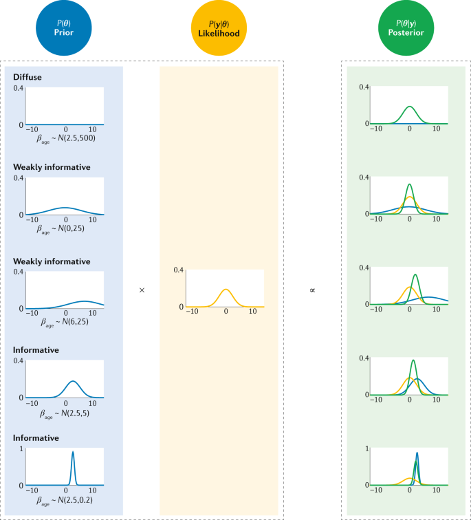
Original figure caption: The prior distribution (blue) and the likelihood function (yellow) are combined in Bayes’ theorem to obtain the posterior distribution (green) in our calculation of PhD delays. Five example priors are provided: one diffuse, two weakly informative with different means but the same variance and two informative with the same mean but different variances. The likelihood remains constant as it is determined by the observed data. The posterior distribution is a compromise between the prior and the likelihood. In this example, the posterior distribution is most strongly affected by the type of prior: diffuse, weakly informative or informative. β age, linear effect of age (years); θ, unknown parameter; P(.), probability distribution; y, data.
Practical example: the Gravity Model
In the above figure, the likelihood function is visualized as independent of the prior distributions. In practice, the likelihood is the way that parameter choices selected from the prior distributions are related to the empirical data. The choice of likelihood represents belief in the distribution governing the system which created the empirical data.
The Basic Gravity Model from the Mobility R package which we used in Call detail record aggregation methodology impacts infectious disease models informed by human mobility gives a simple example of how a likelihood function relates parameter estimates to empirical data. This model has one unknown parameter $\theta$ which scales the gravity equation (based on population sizes and distances between origin and destination locations) to the number of travelers observed in the empirical movement data. The model “is fitted to the movement matrix with a Poisson likelihood link function”.
Here, the choice of the likelihood function is defined by the format of the empirical data. Movement between areas is described by discrete counts of individuals traveling between locations in a fixed time period. This aligns directly with the formulation of the Poisson distribution, which models discrete counts with an average rate $\lambda$.
Here is the code where this happens:
model {
    for (i in 1:length(N_orig)) {
      for (j in 1:length(N_dest)) {
        M[i,j] ~ dpois( theta * ((N_orig[i] * N_dest[j]) / (D[i,j]+0.001)) )
      }
    }
    theta ~ dgamma(0.001,0.001)
}
In this model, the likelihood is defined by the Poisson distribution dpois, with one parameter $\lambda$. This parameter in turn is defined by the equation for the gravity model. Here, dpois is the likelihood function, and theta is a random variable chosen from (in this case) an uninformative prior.
Internally, JAGS computes the simplified version of Bayes' Theorem above, and selects or rejects possible values of $\theta$ given the probability of the parameter choice from the prior, and the likelihood of the parameter choice given the data.
Using different likelihoods
In the above example, the likelihood function is the Poisson distribution. This is convenient because the Poisson distribution is defined by one parameter $\lambda$ meaning that the Gravity equation alone defines the shape of the resulting likelihood distribution.
This raises the question: what about likelihoods defined by more than one parameter? Imagine that we assumed the count of travelers followed a Normal distribution (parameterised by mean $\mu$ and variance $\sigma^2$). In this case, $\mu$ would be defined by the gravity equation and $\sigma^2$ would simply be defined as another random variable tau in the model.
model {
    for (i in 1:length(N_orig)) {
        for (j in 1:length(N_dest)) {
            M[i,j] ~ dnorm(mu[i,j], tau)
            mu[i,j] <- theta * ((N_orig[i] * N_dest[j]) / (D[i,j] + 0.001))
        }
    }
    theta ~ dnorm(0.0, 0.001)
    tau ~ dgamma(0.001, 0.001)
}
Conclusion
In the simplest terms, the likelihood of a model relates parameter choices to the empirical data to which the model is being fit. Higher likelihood for a given set of parameters indicates a higher probability that these parameters generated the observed data. This is combined with the probability of the parameters given the prior parameter distributions, through Bayes' Theorem. A framework like JAGS or Stan will inform its choice of model parameters based on increasing this combined (posterior) probability.
The choice of a likelihood function is like the other choices that have to be made when specifying a bayesian model. It is important to make the decision carefully and consider how the choice of a likelihood may influence the results of your model, just like you would carefully consider your choice of prior distributions.
The examples above helped me improve my understanding of the how a likelihood function fits empirical data together with the parameters of a bayesian model. Hopefully it helps you too!
Sources
Bayesian statistics and modelling (Nature Primer)
Is there any difference between Frequentist and Bayesian on the definition of Likelihood?